Advanced Workflows¶

tranSMART provides the ability to generate the following analyses and visualizations:

Advanced Workflows use the R software environment for statistical computing and to generate analyses and visualizations. For more information, visit http://www.r-project.org.

Running the Analyses¶

To begin to run any analysis:

In Analyze, open the study of interest, or open the Advanced Trials folder to run an analysis of data from multiple studies.
Define the cohort(s) you want to analyze by dragging one or more concepts into empty subset definition boxes. For more information, see Defining the Cohorts.

The following sections describe how to run specific analyses after you perform the above steps.

Optionally, after you run an analysis, you can download the associated R data by clicking Download raw R data below the visualization.

Note

Visualization may take a few seconds to a few minutes to appear.

aCGH Survival Analysis¶

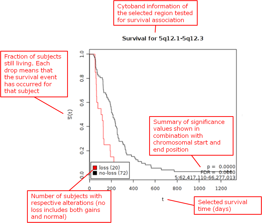
This is a statistical test (logrank) for survival data and called copy number data. The testing is recommended to be performed on high-dimensional data nodes containing chromosomal region information.

To begin the analysis, see Running the Analyses, then perform the following steps.

To perform an aCGH Survival Analysis:

Click the Advanced Workflow tab, then open the Analysis menu.
Select aCGH Survival Analysis.

The Variable Selection section appears.
Define the following variables:
- Region: A high-dimensional data node containing the chromosomal regions.
- Survival Time: A numerical data node containing survival time of interest (for example: Overall Survival [days]).
- Censoring Variable: A categorical data node indicating status subjects in which the selected event in survival time did NOT happen (for example, for Overall Survival Time, the Censoring Variable to select is Alive).
- Alteration type: The type of chromosomal alteration used to test association to survival (gains, losses, both).
- Permutations: The significance of the p-values is evaluated through permutations, and a false discovery rate is calculated. At least 10,000 permutations are recommended for final calculations. This will require a significant amount of time. (Permutations can be lowered for exploratory purposes.)
Click Run Analysis. As this may take a while, users are advised to select the option Run Job in Background in the popup window. The analysis can be retrieved at a later time in the Analysis Jobs tab.
Results appear in two sections:
- The chromosomal regions present in the high-dimensional data node are shown in a table, appended with p-values and false discovery rates.
- You can sort through the chromosomal regions, click on a region of interest and press the button Show Survival Plot. This will plot the survival curve for that particular region (see example below).
You can also opt to click Download Result, in which case both the table and all survival plots are obtained.

Reference: Wiel et al. (2005) “CGHMultiArray: exact p-values for multi-array comparative genomic hybridization data.” Bioinformatics 21: 3193-3194.

Box Plot with ANOVA¶

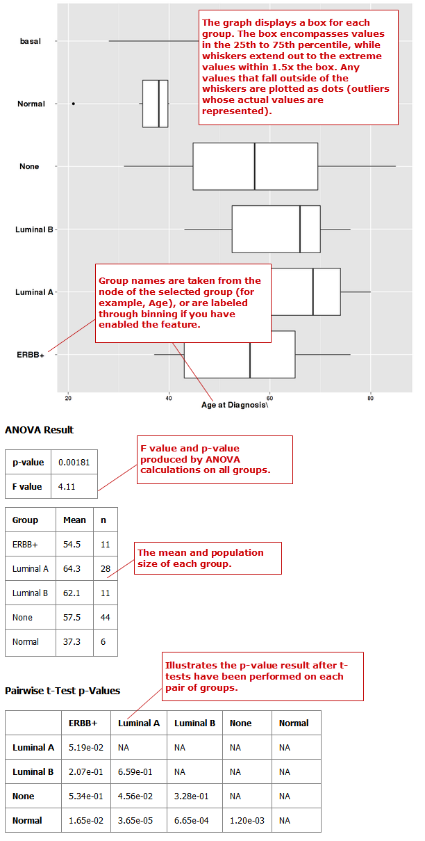
A box plot with ANOVA analysis displays a box and whisker plot with corresponding analysis of variance in the sample(s).

To begin the analysis, see Running the Analyses, then perform the following steps.

To perform a box plot with ANOVA analysis:

Click the Advanced Workflow tab, then open the Analysis menu.
Select Box Plot with ANOVA.

The Variable Selection section appears.
Define an independent variable and a dependent variable, following the instructions above the boxes. You must use one categorical variable and one continuous variable. The boxes are plotted based on the categorical variable:
- If the independent variable is categorical, the boxes are plotted horizontally.
- If the dependent variable is categorical, the boxes are plotted vertically.
- If you select two continuous variables, you must bin one to create a categorical value.
Optionally, enable binning by selecting Enable binning.

Data binning refers to a pre-processing technique used to reduce minor observation errors. Clusters of data are replaced by a value representative of that cluster (the central value). For information on binning, see Data Binning Using Box Plot with ANOVA.
Click Run.

Your analysis appears below:

Correlation Analysis¶

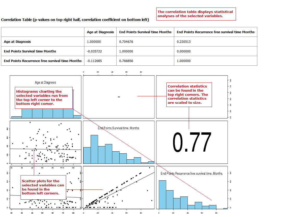
In a correlation analysis, you are using statistical correlation to assess the relationship between variables.

To begin the analysis, see Running the Analyses, then perform the following steps.

To perform a correlation analysis:

Click the Advanced Workflow tab, then open the Analysis menu.
Select Correlation Analysis.

The Variable Selection section appears.
Define two or more continuous (or numerical) variables (for example, Age).
Indicate how you want to run the correlation in the Run Correlation dropdown menu.

Note: At this time, correlations are run by variable only.
Select the analysis you want to perform from the Correlation Type dropdown menu:

Note

The analyses listed under Correlation Type refer to different regression algorithms.
Click Run.

Your analysis appears below:

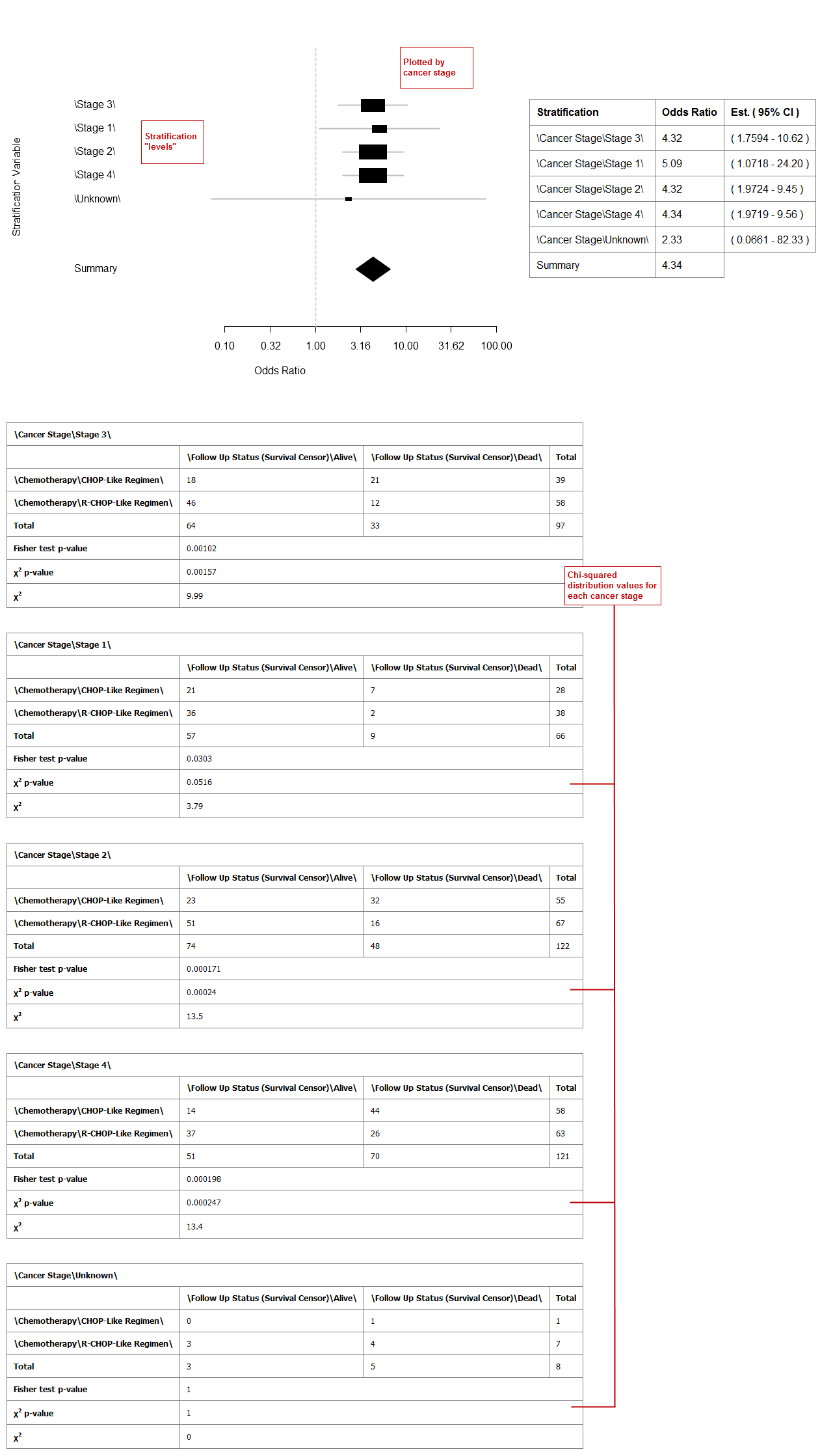
Forest Plot¶

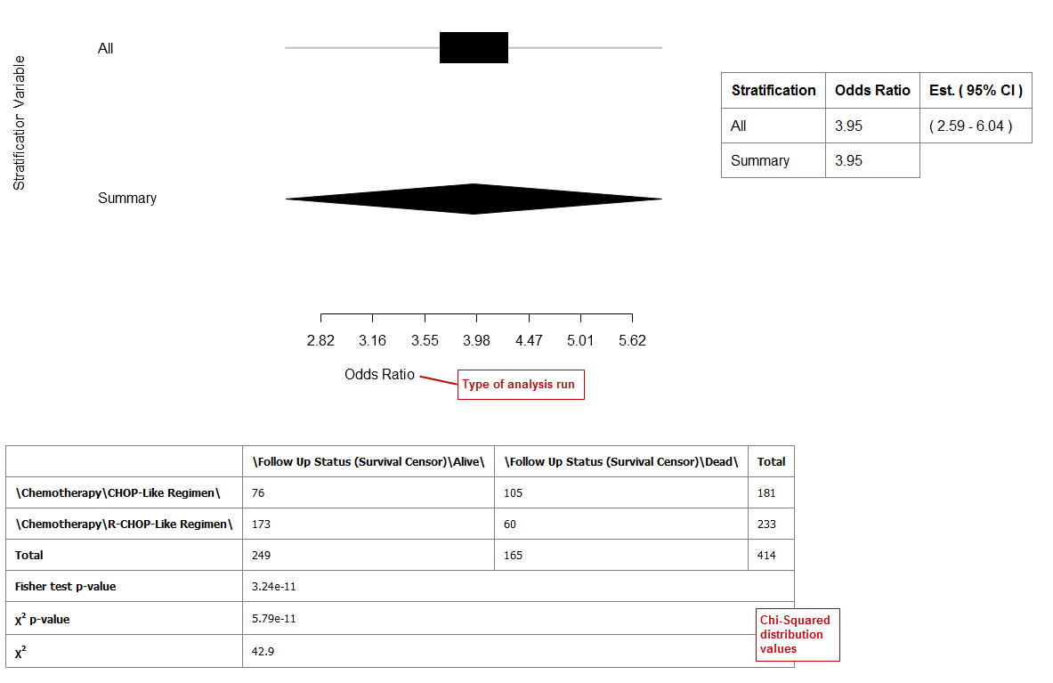
A forest plot graphically displays the relative strength of treatment effects among various cohorts (for example, people who took the same drug). Relative strength can be calculated in two ways:

As relative risk given exposure to a treatment or an environmental factor — that is, the probability of an event occurring in a group of exposed subjects measured against the probability of the event occurring in a group of non-exposed subjects.
As an odds ratio — that is, the odds of an event occurring in one group measured against the odds of an event occurring in a different group.

To begin the analysis, see Running the Analyses, then perform the following steps.

To perform a forest plot analysis:

Click the Advanced Workflow tab, then open the Analysis menu.
Select Forest Plot.

The Variable Selection section appears.
Define the following variables:
- Independent variable: Specifies the experimental or treatment variable being measured in the analysis. If this variable is continuous, it requires binning.
- Control or Reference variable: Indicates the control or reference variable for the analysis; for example, no treatment or placebo. If this variable is continuous, it requires binning.
- Dependent Variable: Indicates the event outcome. Variables entered must be mutually exclusive; for example, Alive and Dead.
  
  If there is only one node in the concept you want to use for Dependent variable, use the checkbox below the box to create the second node. For example, the only node in Gender is Female. tranSMART presumes that each subject for whom Female does not apply is Other.
  
  If this variable is continuous, it requires binning.
- Stratification Variable: Stratifies the relationship between the dependent and independent variables by the variable specified here. For example, if you add the stratification variable Cancer Stage, data is plotted and displayed for each stage. Without stratification, data displays as a single summary value in the graph.
If this variable is continuous, it requires binning.
Optionally, enable binning by clicking the Enable button.

For information, see Data Binning Using Forest Plot.
In Statistic Type, click Odds Ratio or Relative Risk.
Click Run.

Your analysis appears below:

Example 1: Odds Ratio analysis run without stratification:

Example 2: Odds ratio analysis with stratification:

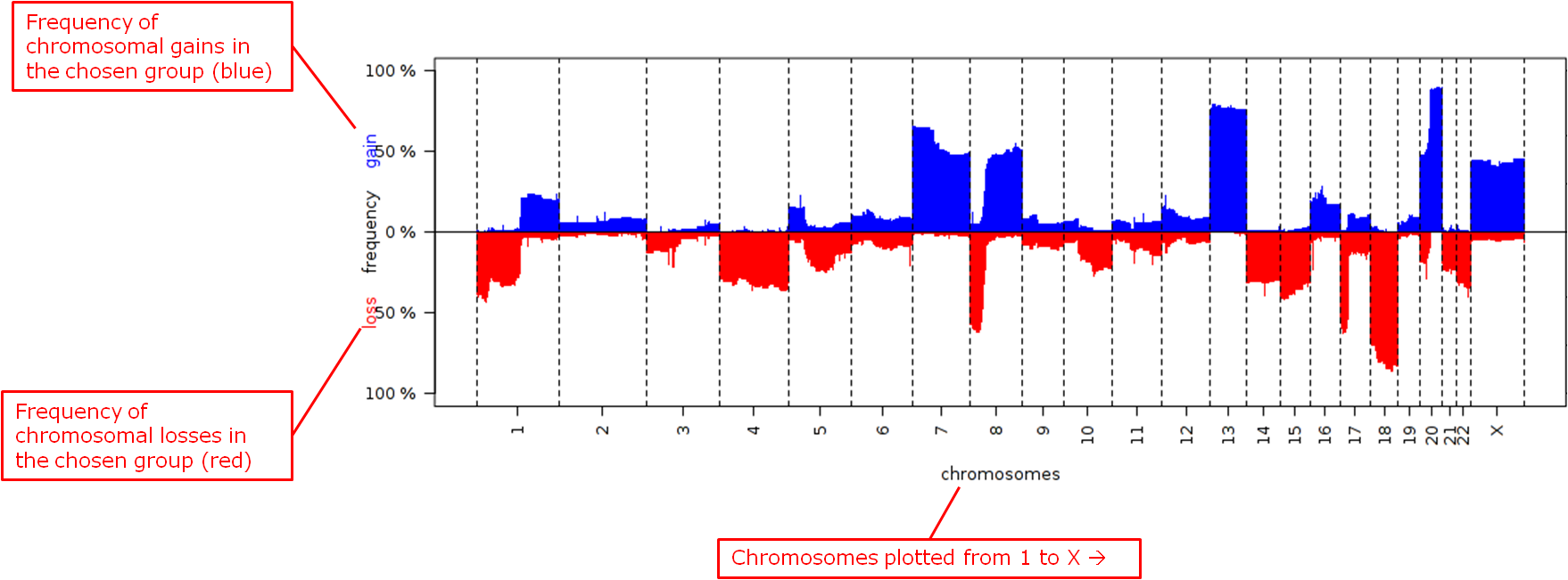
Frequency Plot for aCGH¶

This analysis plots the copy number alteration frequencies for different groups. This analysis is performed on high-dimensional data nodes containing chromosomal region information.

Note

This analysis represents a quick way to investigate alteration frequencies of the selected groups and is very similar to the advanced workflow analysis Group Test for aCGH, in which statistical testing is performed. It is advisable to use the Frequency Plot for aCGH analysis for exploratory purposes before performing statistical testing (which requires a significant amount of time).

To begin the analysis, see Running the Analyses, then perform the following steps.

To perform a Frequency Plot for aCGH analysis:

Click the Advanced Workflow tab, then open the Analysis menu.
Select Frequency Plot for aCGH.

The Variable Selection section appears.
Define the following variables:
- ArrayCGH: A high-dimensional data node containing the chromosomal regions.
- Group: Categorical data nodes separating the samples into two or more groups (though only one group may be plotted as well).
Click Run Analysis.
Result

Frequency plots of copy number alterations in each defined group are shown. Frequencies of chromosomal gains are in blue and chromosomal losses are in red.

Example of a plot of one group:

Reference: Mark A. van de Wiel, Kyung In Kim, Sjoerd J. Vosse, Wessel N. van Wieringen, Saskia M. Wilting and Bauke Ylstra. ” CGHcall: calling aberrations for array CGH tumor profiles.” Bioinformatics, 23, 892-894.

GenePrint¶

The Geneprint provides a visual summary of notable features across different datatypes. These features include mRNA expression (up/down regulation based on threshold), protein expression (up/down regulation based on threshold), aCGH copy number aberrations (loss, normal, gain, amplified), vcf small genomic variants (indication of mutation or not).

To begin the analysis, see Running the Analyses, then perform the following steps.

To perform a Geneprint analysis:

Click the Advanced Workflow tab, then open the Analysis menu.
Select Geneprint

The Variable Selection section appears
Drag a high-dimensional data node into the Variable Selection box. The data node may be mRNA, protein, aCGH (copy number aberrations) or vcf (small genomic variants) data. It is possible to drag multiple nodes of different types into the box.
Click the High Dimensional Data button.

The Compare Subsets-Pathway Selection dialog box appears
Select one or more Genes/Pathways/mirIDs/UniProtIDs by typing in their symbols and selecting them from the list.
Click ‘Apply Selections’.
Specify thresholds for the mRNA and/or protein expression z-scores (if applicable).
Click Run.

Your analysis appears below

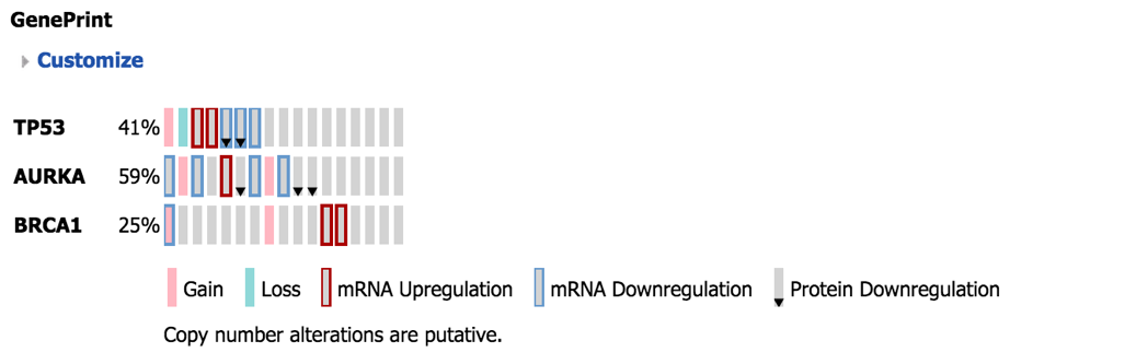
Explanation of Geneprint result:

The geneprint shows a glyph (rectangle) for each gene-subject pair. Each row represents a gene, each column a subject. The columns are sorted by feature, starting at the first gene. Each glyph represents the data values using color coding and icons. An explanation of these is provided in the legend.

In order for data to be compatible with Geneprint, the patient/subject ids for the different data types must match to show them in the same columns, and gene information must have been loaded in the database for all data types.

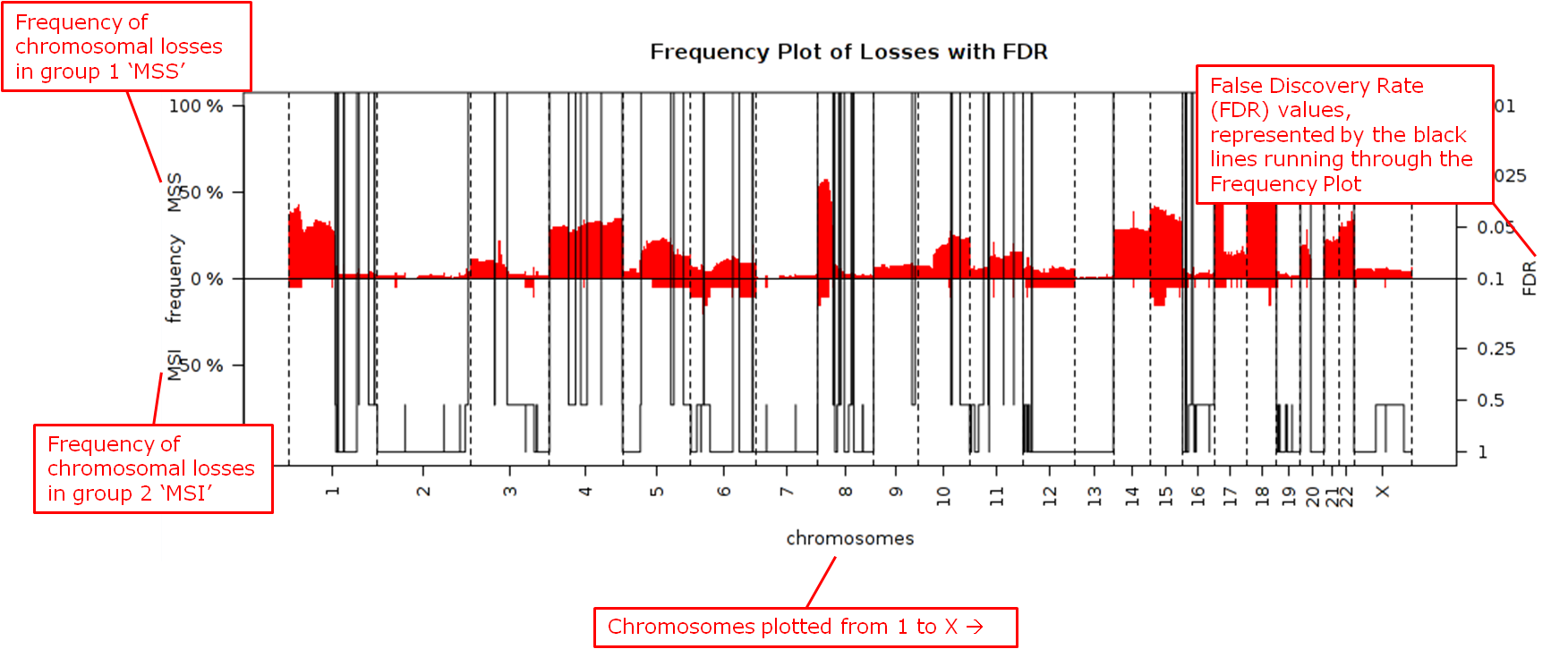
Group Test for aCGH¶

Three different statistical tests are available to determine potential differences in status of copy number alterations between various groups. The testing is recommended to be performed on high-dimensional data nodes containing chromosomal region information.

This analysis plots the copy number aberration frequencies for different groups and indicates significant different regions between these groups.

To begin the analysis, see Running the Analyses, then perform the following steps.

To perform a Group test for aCGH analysis:

Click the Advanced Workflow tab, then open the Analysis menu.
Select Group Test for aCGH.

The Variable Selection section appears.
Define the following variables:
- Region: A high-dimensional data node containing the chromosomal regions.
- Group: Categorical data nodes separating the samples into two or more groups.
- Statistical Test: Select the test to perform:
  - Chi-square: Test for the association between alteration pattern and group label. Supports multiple comparisons.
  - Wilcoxon: Rank-sum test for two groups.
  - Kruskal-Wallis: Generalization for Wilcoxon for more than two groups.
- Alteration type: The type of chromosomal alteration used to test the association (gains, losses, both).
- Permutations: The significance of the p-values is evaluated through permutations, and a false discovery rate is calculated. At least 10,000 permutations are recommended for final calculations. This will require a significant amount of time. (Permutations can be lowered for exploratory purposes in lieu of generating a Frequency Plot for aCGH.)
Click Run Analysis. As this may take a while, consider selecting the option Run Job in Background in the popup window. The analysis can be retrieved at a later time in the Analysis Jobs tab.
Results appear in two sections:
- The chromosomal regions present in the high-dimensional data node are shown in a table, appended with p-values and false discovery rates.
- Frequency plots of copy number alterations in each defined group are shown. In particular, “Mirror frequency plots” are shown; for example:

Reference: Wiel et al. (2005) “CGHMultiArray: exact p-values for multi-array comparative genomic hybridization data.” Bioinformatics 21: 3193-3194.

Group Test for RNASeq¶

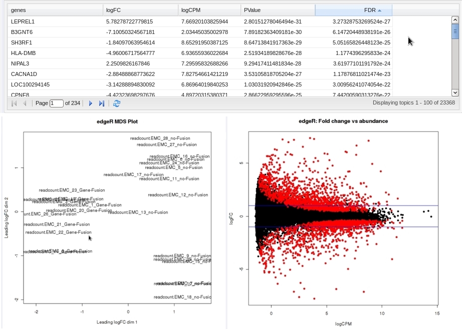
For microarrays, the abundance of a particular transcript is measured as a fluorescence intensity, effectively a continuous response, whereas for digital gene expression (DGE) data the abundance is observed as a count. One of the fundamental data analysis tasks, especially for gene expression studies, involves determining whether there is evidence that counts for a transcript or exon are significantly different across experimental conditions. The software package edgeR (empirical analysis of DGE in R), which forms part of the Bioconductor project, is designed to examine differential expression of count-based expression data between two or more groups.

The Group Test for RNASeq analysis is recommended to be performed on high-dimensional data nodes containing RNASeq-based read count observations. The results of the analysis comprise an ordered table of the differentially expressed genes (or tags, or exons, etc.) and plots visualizing the level of (dis)similarity of individual samples (MDS plot) as well as the DGE data (MA plot).

To begin the analysis, see Running the Analyses, then perform the following steps.

To perform a Group Test for RNASeq analysis:

Click the Advanced Workflow tab, and then open the Analysis menu.
Select Group Test for RNASeq.

The Variable Selection section appears.
Define the following variables:
- RNASeq: A high-dimensional data node containing RNASeq-based read count data.
- Group: Categorical data nodes separating the samples into two or more groups.
- Analysis Type: Select the type of analysis to perform:
  - two group unpaired
  - multi-group
Click Run Analysis. As this may take a while, consider selecting the option Run Job in Background in the popup window. The analysis can be retrieved at a later time in the Analysis Jobs tab.
Results appear in two sections:
- An ordered table of the differentially expressed genes (or tags or exons, etc.) including fault changes, abundances, p-values, and false discovery rates.
- An MDS plot visualizing the level of (dis)similarity of individual samples, and an MA plot (fold change versus abundance) visualizing the RNASeq data.

Reference: Mark D. Robinson, Davis J. McCarthy and Gordon K. Smyth (2009) “edgeR: a Bioconductor package for differential expression analysis of digital gene expression data.” Bioinformatics (2010) 26 (1): 139-140.

Heatmaps¶

In Analyze, a heatmap is a matrix of data points for a particular set of biomarkers, such as genes, at a particular point in time and/or for a particular tissue sample in the study, as measured for each subject in the study.

In an Analyze heatmap:

The values in the heatmap are based on the Z-score calculation
The color red indicates higher-than-normal expression
The color green indicates lower-than-normal expression
Biomarkers appear in the y-axis, and subjects appear in the x-axis.

Note

A heatmap can display data points for up to 1000 samples.

Max rows to display¶

The order of data points to be display is determined by the standard deviation on probe level. First, the probes that do not have a standard deviation are removed. Then, the standard deviation is calculated independently from groups, so the whole mRNA data set is used. Next the standard deviation values are sorted from the highest to the lowest and only the top rows will be displayed.

Selecting biomarker subsets¶

When using the High Dimensional Data button to select only the biomarkers of interest it is possible selected biomarkers are not displayed in the heatmap image. This is due the dataset of interest not having any data for the selected biomarker.

Note

The autocomplete in the High Dimensional Data pop-up uses biomarker dictionaries to suggest autocomplete. These dictionaries do not take into considerations which biomarkers are available for a selected dataset.

Analyze uses the R software environment for statistical computing and to generate analyses and visualizations. For more information, visit http://www.r-project.org.

You can generate the following types of heatmaps:

Standard Heatmap
Hierarchical Clustering
K-Means Clustering
Marker Selection

Standard Heatmap¶

A standard heatmap is a visualization of biomarker data points with no indication of patterns, groupings, or differentiation among the data points.

To begin the analysis, see Running the Analyses, then perform the following steps.

To perform a standard heatmap analysis:

Click the Advanced Workflow tab, then open the Analysis menu.
Select Heatmap.

The Variable Selection section appears.
Drag a high-dimensional data node (), or several high-dimensional nodes in the case of serial data, into the Variable Selection box.
Click the High Dimensional Data button.

The Compare Subsets-Pathway Selection dialog box appears.
Specify the platform and other filters for the analysis.

For information, see High Dimensional Data.
Click Apply Selections.
In Max rows to display, type the maximum number or rows in the heatmap.
Optionally, select either or both of the following:
Click Run.
Your analysis appears below:

Note

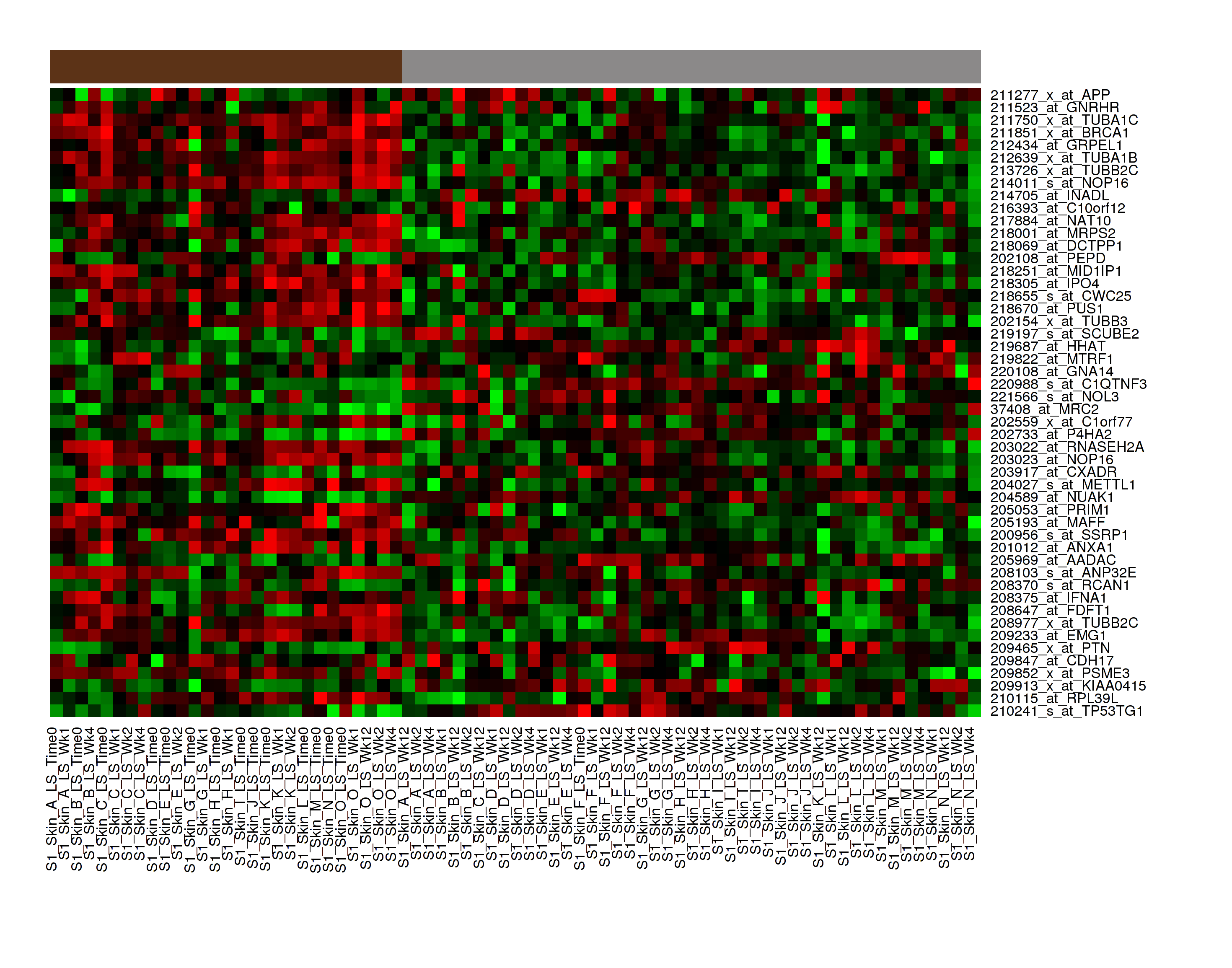
With serial data, the heatmap will display the various conditions ordered by increasing associated value, such as in chronological order for a time series.

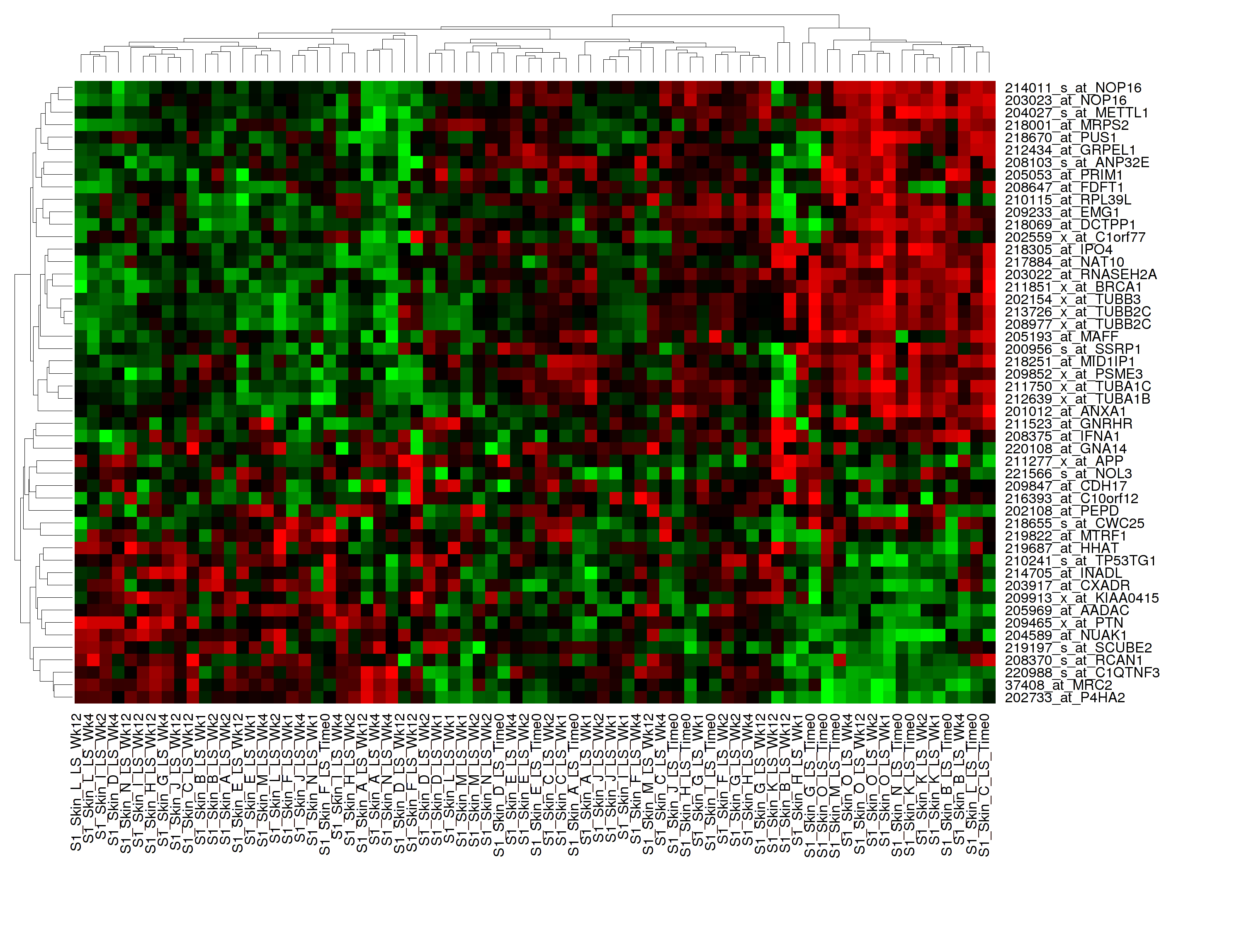
Hierarchical Clustering¶

Hierarchical clustering is a visualization of patterns of related data points in gene expression data.

To begin the analysis, see Running the Analyses, then perform the following steps.

To perform a hierarchical clustering heatmap analysis:

Click the Advanced Workflow tab, then open the Analysis menu.
Select Hierarchical Clustering.

The Variable Selection section appears.
Drag a high-dimensional data node () into the Variable Selection box.
Click the High Dimensional Data button.

The Compare Subsets-Pathway Selection dialog box appears.
Specify the platform and other filters for the analysis.

For information, see High Dimensional Data.
Click Apply Selections.
In Max rows to display, type the maximum number or rows in the heatmap.
Optionally, select one or more of the following:
Click Run.
Your analysis appears below:

Note

To read more about Hierarchical Clustering, visit: http://www.ics.uci.edu/~eppstein/280/cluster.html

K-Means Clustering¶

K-Means clustering is a visualization of groupings of the most closely related data points, based on the number of groupings you specify.

Note

The K-Means analysis clusters columns only. Rows are not clustered.

To begin the analysis, see Running the Analyses, then perform the following steps.

To perform a k-means clustering heatmap analysis:

Click the Advanced Workflow tab, then open the Analysis menu.
Select K-Means Clustering.

The Variable Selection section appears.
Drag a high-dimensional data node () into the Variable Selection box.
Click the High Dimensional Data button.

The Compare Subsets-Pathway Selection dialog box appears.
Specify the platform and other filters for the analysis.

For information, see High Dimensional Data.
Click Apply Selections.
In Number of clusters, type the number of clusters to include in the heatmap.
In Max rows to display, type the maximum number or rows in the heatmap.
Optionally, select Calculate z-score on the fly.
Click Run.
Your analysis appears below. Clusters are represented by the colored bars at the top of the heatmap:

Note

To read more about K-Means Clustering, visit: http://www.ics.uci.edu/~eppstein/280/cluster.html

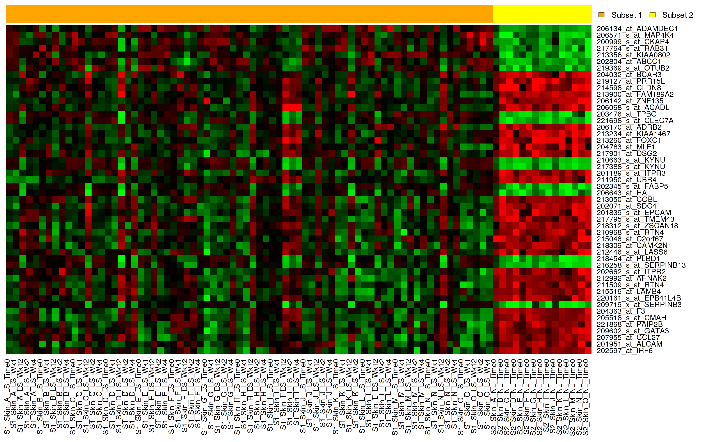
Marker Selection¶

A marker selection heatmap is a visualization of differentially expressed genes in distinct phenotypes. Specifically, the algorithm determines the set of genes which is most differently expressed between the two subsets. This list of differentially expressed genes is subsequently presented in a table, along with a variety of accompanying statistics.

Optionally, you can run a MetaCore Enrichment Analysis from a generated Marker Selection heatmap.

To begin the analysis, see Running the Analyses, then perform the following steps.

Note

Two subsets must be specified when using a Marker Selection heatmap.

To perform a marker selection heatmap analysis:

Click the Advanced Workflow tab, then open the Analysis menu.
Select Marker Selection.

The Variable Selection section appears.
Drag a high-dimensional data node () into the Variable Selection box.
Click the High Dimensional Data button.

The Compare Subsets-Pathway Selection dialog box appears.
Specify the platform and other filters for the analysis.

For information, see High Dimensional Data.
Click Apply Selections.
In the Number of Markers field, type a numeric value. This will determine the number of differentially expressed genes that are returned.
Optionally, select either or both of the following:
Click Run.
Your analysis appears below. The subsets are represented by the colored bars at the top of the heatmap:

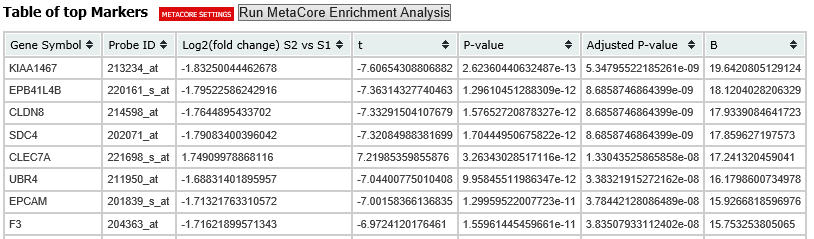
A table of the top markers appears below the heatmap. You can sort the table by clicking any of the column headings. Optionally, you can view MetaCore settings and run a MetaCore Enrichment Analysis by clicking the buttons above the table.

For more information about MetaCore Enrichment Analysis see MetaCore Enrichment Analysis.

The following table represents a portion of the data from the Marker Selection heatmap illustrated above:

Note

For more information on the analyses used in Marker Selection, visit: http://mathworld.wolfram.com/BonferroniCorrection.html

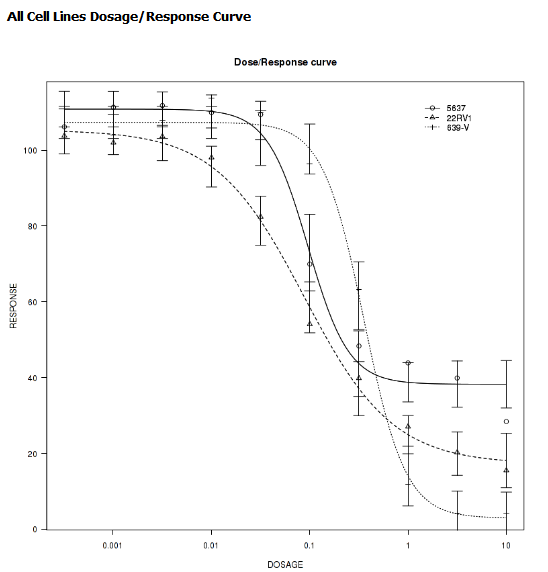
IC50 Dose Response Curve¶

IC50 dose response curve analyses measure the effectiveness of a compound in inhibiting certain biological processes.

To begin the analysis, see Running the Analyses, then perform the following steps.

To perform an IC50 dose response curve analysis:

Click the Advanced Workflow tab, then open the Analysis menu.
Select IC50.

The Variable Selection section appears.
Define the following variables:

Cell Lines

The categorical value that represents the cell lines to plot.

Concentration Variable

The continuous variable that represents the dosage of a compound at a given concentration level.
Click Run.

Your analysis appears below:

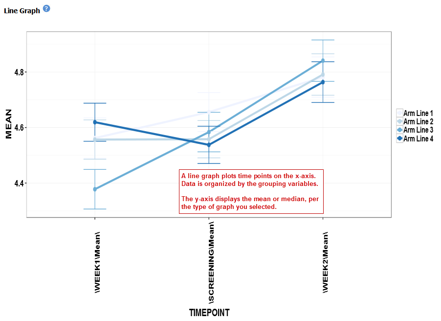
Line Graph¶

A line graph is designed to plot serial numeric data (high or low dimensional); that is, a numeric variable that has been measured in a series of conditions for each subject (for example, several timepoints). For more information on serial data, see Serial Numeric Data.

In a line graph, the various conditions are plotted along the x-axis, at scale (unless you check the Plot evenly spaced option) when the conditions are associated with a numeric value. For example, time series data will be plotted on scale with time.

For categorical conditions, data points are evenly spaced along the x-axis.

The measurement of interest can be plotted for one or several groups (for example, treatment groups) of the defined subsets.

Note

Each group will be plotted as a distinct line on the graph, unless you select Plot individuals as the graph type. In that case, each individual is plotted as a distinct line, using different colors for each group.

To begin the analysis, see Running the Analyses, then perform the following steps.

To perform a line graph analysis:

Click the Advanced Workflow tab, then open the Analysis menu.
Select Line Graph.

The Variable Selection section appears.
Drag and drop several nodes of serial data into the Time/Measurement Concepts selection box. To define the groups, drag and drop nodes into the Group Concepts selection box.

If no group concept is defined, the defined subsets are used as one group.

Note

The order of the data points along the x-axis is controlled by the value defining each condition, even with the Plot evenly spaced option selected; for example, in chronological order for time series.
If you included high dimensional data in either concept box, click the High Dimensional Data button for that box.

The Compare Subsets-Pathway Selection dialog box appears.

Specify the platform and other filters for the analysis.

For information, see High Dimensional Data.
Click Apply Selections.
Optionally, select one or both of the following:
In Graph Type, select the type of line graph you want to display.
Click Run.

Your analysis appears below:

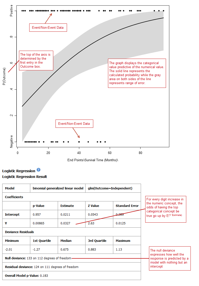
Logistic Regression¶

Logistic regression is a type of regression analysis used to predict the outcome of a variable that can take on a limited number of categories based on one or more predictors. A logistic regression analysis displays a categorical value predictive of a numerical value.

To begin the analysis, see Running the Analyses, then perform the following steps.

To perform a logistic regression analysis:

Click the Advanced Workflow tab, then open the Analysis menu.
Select Logistic Regression.
The Variable Selection section appears.
Define the Independent Variable and the Outcome variables, following the instructions above the entry boxes.

Note

The categorical Outcome variable must use two — and only two — nodes.

The top of the logistic regression plot is determined by the first entry in the Outcome variable box.
Optionally, select Enable binning.
Click Run.

Your analysis appears below. Note that raw data (Event/Non-Event data) is plotted along the top and bottom of the analysis.

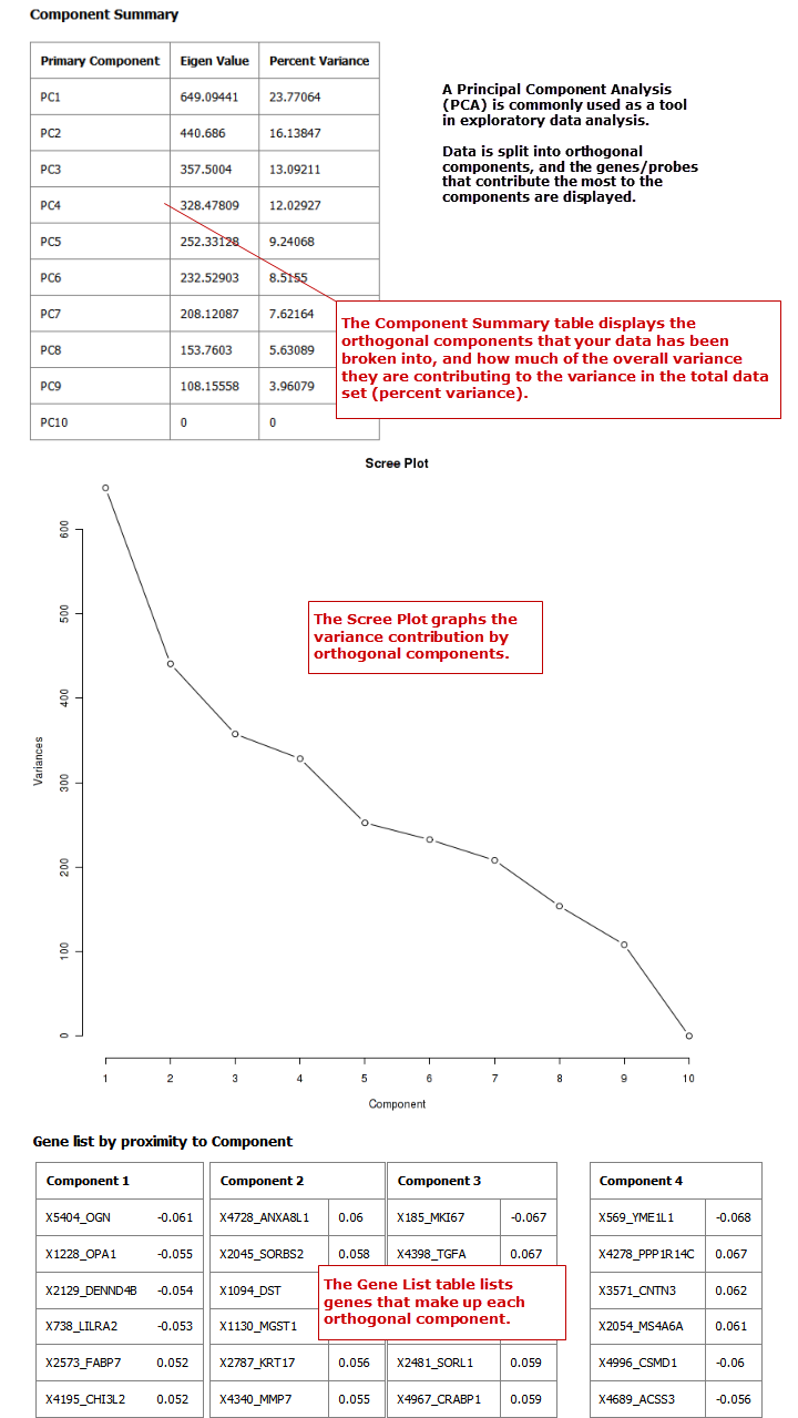
PCA¶

In a principal component analysis (PCA), the total number of variables in the dataset is reduced to a smaller number of variables – the principle components of the dataset.

Principal component variables are calculated from correlated variables in the total dataset. In other words, the principal component analysis is a workflow used to identify variance in a dataset. The analysis can be run on an entire microarray chip, or on a pathway.

To begin the analysis, see Running the Analyses, then perform the following steps.

Note

Only one subset may be specified in this analysis. Information in Subset 2 will be ignored.

To perform a PCA analysis:

Click the Advanced Workflow tab, then open the Analysis menu.
Select PCA.

The Variable Selection section appears.
Drag a high-dimensional data node () into the Variable Selection box.
Click the High Dimensional Data button.

The Compare Subsets-Pathway Selection dialog appears.
Specify the platform and other filters for the analysis.

For information, see High Dimensional Data.
Click Apply Selections.
Optionally, select either or both of the following:
Click Run. Your analysis appears below:

Note

For more information regarding PCAs, see: http://psb.stanford.edu/psb-online/proceedings/psb00/raychaudhuri.pdf.

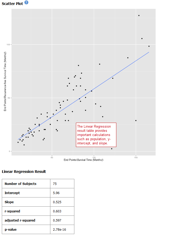
Scatter Plot with Linear Regression¶

A scatter plot displays values for two variables within a dataset, with a line that best fits the slope of the data.

To begin the analysis, see Running the Analyses, then perform the following steps.

To perform a scatter plot with linear regression analysis:

Click the Advanced Workflow tab, then open the Analysis menu.
Select Scatter Plot with Linear Regression.

The Variable Selection section appears.
Define an independent variable and a dependent variable. Both variables should be continuous (for example, Age) and can be high dimensional data.
If you included high dimensional data in either variable box, click the High Dimensional Data button for that box.

The Compare Subsets-Pathway Selection dialog box appears.

Specify the platform and other filters for the analysis.

For information, see High Dimensional Data.
Click Apply Selections.
Click Run.
Your analysis appears below:

Log₁₀ Transformation¶

Often there will be a large spread between values in the x-axis of a scatter plot analysis. You can use the log₁₀ option to transform the values in the x-axis, making the graph easier to analyze.

To use the log₁₀ transformation:

Select the study you want to use and drag it into a Subset Definition box.
Select the Scatter Plot with Linear Regression analysis.
Enter the independent and dependent variables.
Check the box next to Perform log10 transformation on independent variable (below the Independent Variable box):
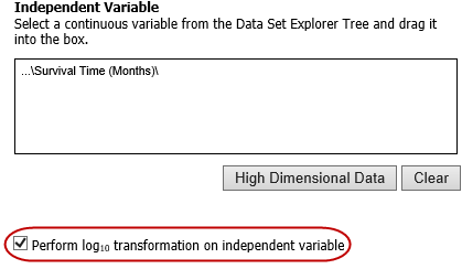
Click Run. Your analysis appears below:

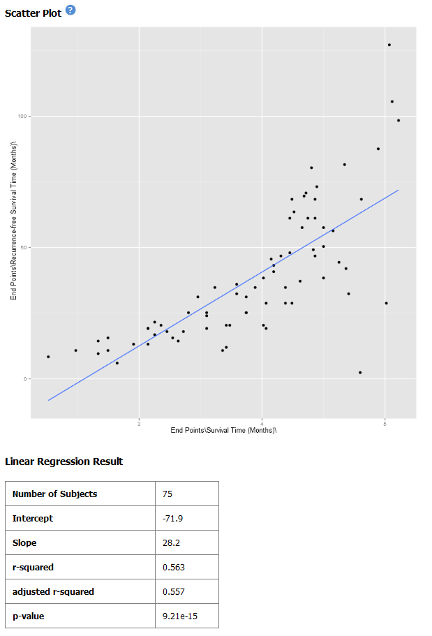
Note

The difference between the x-axis on the scatter plot shown previously (no log₁₀ transformation) and the graph shown immediately above. On the first graph, the x-axis values are plotted by multiple of 50 — 50, 100, 150. When the log₁₀ transformation is applied, the x-axis values are plotted per much lower values — 3, 4, and
The Linear Regression Result values reflect the recalculated data.

Survival Analysis¶

A survival analysis displays time-to-event data.

To begin the analysis, see Running the Analyses, then perform the following steps.

To perform a survival analysis:

Click the Advanced Workflow tab, then open the Analysis menu.
Select Survival Analysis.

The Variable Selection section appears.
Define the following variables:
- Time: A numerical measure of duration; for example, Overall Survival Time (Years).
- Category: The groups into which the data will be split in order to compare the time measured; for example, Cancer Stage. This variable is optional. If you do use it, you must enter two nodes for the comparison.
If this variable is continuous, it requires binning.
- Censoring Variable: Specifies which patients had the event whose time is being measured. For example, if the Time variable selected is Overall Survival Time (Years), an appropriate event variable is Alive.
Optionally, select Enable binning.

For details, see Data Binning Using Survival Analysis.
Click Run.

Your analysis appears below:

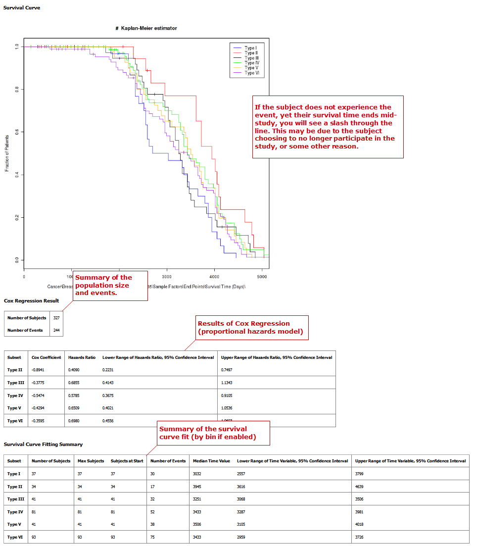
Table with Fisher Test¶

A Fisher Test analysis examines the significance of associated categorical variables.

To begin the analysis, see Running the Analyses, then perform the following steps.

To perform a table with fisher test analysis:

Click the Advanced Workflow tab, then open the Analysis menu.
Select Table with Fisher Test.

The Variable Selection section appears.
Define independent and dependent variables, following the instructions over the Independent Variable and Dependent Variable boxes.
If you included high dimensional data in either variable box, click the High Dimensional Data button for that box.

The Compare Subsets-Pathway Selection dialog box appears.

Specify the platform and other filters for the analysis.

For information, see High Dimensional Data.
Click Apply Selections.
Optionally, select Enable binning.

If you select this option, the first, or top, variable in the Dependent Variable box will be used as the conditional variable to calculate the binary outcome. Multiple variables can be categorized into two distinct groups by enabling the Data Binning option. The variable selected in Bin 1 will be used as the conditional variable to calculate the binary outcome.

For information on binning with this type of analysis, see Data Binning Using Table with Fisher Test.
Click Run.
Your analysis appears below:

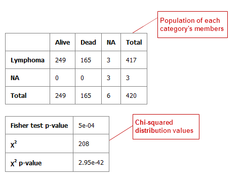
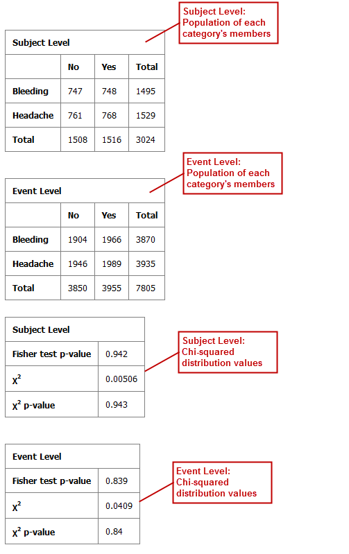
Table with Fisher Test with Linked Events¶

If you run the Table with Fisher test analysis using linked events data, the analysis contains two levels for each portion of the analysis: subject-level and event-level.

Using a linked event study, define your variables as described above the Independent Variable and Dependent Variable boxes. Then click Run to create the analysis.

Note that there are now two sets of results for each type of data presented.

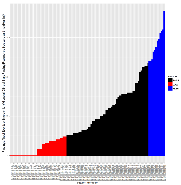
Waterfall Plot¶

A waterfall plot displays a bar chart where a single bar represents each sample in a cohort. Bars are sorted by selected variables and displayed in ascending order. You can further refine the display by specifying ranges that will shade bars accordingly.

To begin the analysis, see Running the Analyses, then perform the following steps.

To generate a waterfall plot:

Click the Advanced Workflow tab, then open the Analysis menu.
Select Waterfall.

The Variable Selection section appears.
Define the required variable by selecting a continuous data node from the Dataset Explorer tree and dragging it into the Data Node definition box:

Note

Continuous data nodes are indicated by the (123) icon to the left of study data.
In Low Range, select the appropriate operator from the dropdown menu, then type the value of the low range.
In High Range, select the appropriate operator from the dropdown menu, then type the value of the low range.
Optionally, if you would like the variable, as well as the specified ranges, to appear within separate subsets in the Comparison tab, click Select inputs as Cohort.
Click Run.
Your analysis appears below:

High Dimensional Data¶

The High Dimensional Data button available within the Advanced Workflow section of Analyze allows you to specify additional inputs for selected variables. These inputs help filter specific information of value (such as platforms, samples, and genes or pathways).

Note

The High Dimensional Data feature must be used when you perform an analysis using high dimensional data (such as SNP, gene expression, RBM, etc.) symbolized by the DNA icon ( ). Additionally, the High Dimensional Data feature cannot be used without high dimensional data.

When you click the High Dimensional Data button while setting up an analysis, the Compare Subsets-Pathway Selection dialog box appears. tranSMART will attempt to pre-populate default values in the associated fields of the dialog box based on the underlying data in the variable selection box.

The dialog box has the following filters:

Marker Type

The platform type (for example, Gene Expression, SNP, mRNA, etc.) used to collect biomarker data in the study.

GPL Platform

The specific name of the platform used in the study.

Sample

The type of sample tested in the study.

Tissue

The type of tissue tested in the study.

Select a Gene/Pathway/mirID/UniProtID

The gene or other item of interest. Separate multiple entries with a comma.

If you would like to run the analysis on the entire chip, leave this field blank.

Aggregate Probes?

The checkbox can be selected if the variable chosen is either gene expression data or SNP copy number data.

If the checkbox is selected, the algorithm WGCNA (weighted correlation network analysis) is employed. For genes that are comprised of multiple probes, WGCNA selects the probe that best represents the overall expression level or copy number.

This checkbox does not apply to all advanced workflows.

Note

WGCNA was developed by the Department of Human Genetics at UCLA. For more information, see http://www.genetics.ucla.edu/labs/horvath/CoexpressionNetwork/.

When finished defining the filters, click Apply Selections, then continue setting up the analysis in the Variable Selection section.

Data Binning¶

Data binning refers to a pre-processing technique used to reduce observation errors and to allow continuous variables to become categorical. Clusters of data are replaced by a value representative of that cluster (the central value).

Note

The data displayed after binning represents the data available in the study. If, for example, you have selected to bin based on date range (0-10 years of age), yet there is only data available for subjects eight years old and up, the bin will display the age range as 8-10.

Data binning caveats¶

Implementation of the automatic binning causes in issues in some cases. Here we detail an example for both the Evenly distributed population (EDP) and Evenly spaced bins options using the DeCoDe_WP5_demo study.

Variables used:

\DeCoDe_WP5_demo\..\Age\ (continuous)
\DeCoDe_WP5_demo\..\Number of first degree relatives with cancer diagnosis\ (discrete)

Steps for Evenly Distributed Population binning:

Checks if manual binning is enabled, if not executes
Uses the binning variable to create bins, if the variable is categoric makes use or nominal representation (Factors) to type cast to numeric.
Determine how many subjects per bin by dividing the total number of patients by number of bins.
Sort the binning column.
Set the starting and ending row number
Loop over all the bins but the last one and assign a bin number based on the sorted result
Checks if there are other values in the binning column that are equal to the first row of the current bin, if so assign them to the same bin.
This last step is where it screws up when you have a weird distribution in your data. The second concept used for binning (Number of first degree relatives with cancer diagnosis) has this distribution:

Original value overview:

Value 0 1 2 3

Counts 120 14 4 2

Which gives the following bins:

Bin 1 2 3 4

Counts 70 35 0 35

Combined to see which values are in which bins:

Value 0 1 2 3

Bin

1 70 0 0 0

2 35 0 0 0

3 0 0 0 0

4 15 14 4 2

This gives weird results as you can see.

In this particular case if you run this example in tranSMART you will only see 2 bins instead of 4. That is because of the next piece of code that names the bins. The logic tries to be smart in finding the smallest value from the next bin but as you see the first bins only have 0 values in the bins screwing up the logic and basically returning 2 labels. These labels are then set as the bins and are returned to the analysis to use as groups.

If you turn around the variables and use Age to do the binning it works fine and gives the expected results:

Bin	1	2	3	4
Counts	36	35	34	35

The reason this is happening is due to the following block of code when data is skewed and discrete.

# If any row in any bin has a value that matches the
# first row in this bin, add those rows to the previous bin.
if(i>1) {
    valuesInPreviousBins = (dataFrame[[binningColumn]]==dataFrame[[binningColumn]][binStart])
    dataFrame$bins[
        valuesInPreviousBins & (dataFrame$bins==i)
        ] = i-1
    }

What happens for this example above is the following:

Code goes through first loop and assigns bin number 1 based on binStart and binEnd parameters.
Second iteration the bin number is larger than 1 so an additional statement updates the binStart to binStart + binSize.
The bin number 2 is assigned based on binStart and binEnd again.
Check if the first value of the bin is also in the previous bin, if so, adjust bin number to 1 (line of code above). NOTE! this is only done for the current bin we are looking at.
This is repeated for all bins except the last.
The last bin is assigned to all bins that did not have a bin assigned yet.
In our case this goes wrong because the 0 value is 85% of our subjects. Due to this heavy.
Skew the code breaks as it does not cover this assumption.

Data Binning Using Box Plot with ANOVA¶

When conducting a Box Plot with ANOVA analysis, at least one of the variables selected should be a continuous variable (for example, age), and the other should be a categorical value (for example, tumor stage).

A continuous variable can be viewed as a categorical value using the binning feature, described below. Alternatively, binning can be used to regroup categorical data to consider it as a single variable. For example, if histological grade with values such as Well Defined, Moderately Well Defined, and Poorly Defined are selected, you can group Moderately Well Defined with Poorly Defined and treat them as one group for the purposes of this analysis.

To use the data binning feature with a box plot analysis:

Begin to set up a Box Plot with ANOVA analysis by following the instructions in section Box Plot with ANOVA.
Enable binning by selecting Enable binning.
Define the following and then click Run.
Variable

Select which variable should define the groups (Independent or Dependent) from the dropdown menu.

If the independent variable defines the groups, boxes will be plotted horizontally. If the dependent variable defines the groups, boxes will be plotted vertically

Variable Type

Select whether the variable you have defined above is continuous or categorical from the dropdown menu.

A continuous variable can be turned into a categorical variable when you use the binning feature.

Number of Bins

Type the number of bins you would like data to be organized in.

This step may require trial and error based on how you want to display data.

Bin Assignments
Select how you would like data to be binned from the dropdown menu.

Note

This feature can only be used when the variable type selected above is continuous.

What to use when:
- Evenly Distribute Population: Assigns bins based on the underlying data.
  
  For example, if the majority of the subjects in the study were elderly, bins based on age could look like: [(1-40), (40-80), (81-85), (86-90), (90-92)].
- Evenly Spaced Bins: Creates bins based on the overall range of the variable.
  
  For example, if the majority of the subjects in the study were elderly, bins based on age could look like: [(1-20), (21-40), (41-60), (61-80), (81-100)].
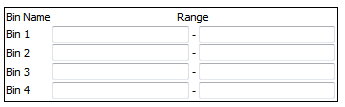
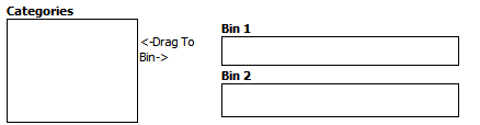
Manual Binning
Select the checkbox if you want to bin manually.

Note

This is the only binning method available if you are trying to bin a categorical variable type.

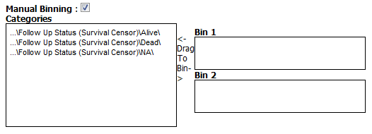
Complete the binning form that populates as a result of checking the Manual Binning box.
- For continuous data:
- For categorical data:

Data Binning Using Forest Plot¶

Data binning is used in forest plot analyses if the variable you want to use is continuous (for example, age) but needs to be viewed as categorical data. As an alternative, binning can be used to regroup categorical data to consider it as a single variable. For example, if histological grade with values such as Well Defined, Moderately Well Defined, and Poorly Defined are selected, you can group Moderately Well Defined with Poorly Defined and treat them as one group for the purposes of this analysis.

To use the data binning feature with a forest plot analysis:

Begin to set up a Forest Plot analysis by following the instructions in section Forest Plot.
Enable binning by clicking the Enable button.
Define the following and then click Run.
Variable

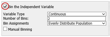
Select the variable(s) you want to bin by checking the Bin the [*variableType*] Variable box next to the appropriate variables.

You can bin from none to all four variables.

Example for binning an independent variable:

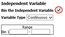
Variable Type

Select whether the variable you have defined above is continuous or categorical from the dropdown menu.

A continuous variable can be turned into a categorical variable when you use the binning feature.

Number of Bins

Used with the Dependent and Stratification Variables only.

Enter the number of bins into which you would like data to be organized.

This step may require trial and error based on how you want to display data.

Bin Assignments
Select how you would like data to be binned from the dropdown menu.

Note

This is only an option when binning a continuous variable in the Dependent or Stratification input boxes.

When to use what:
- Evenly Distribute Population: Assigns bins based on the underlying data.
  
  For example, if the majority of the subjects in the study were elderly, bins based on age could look like: [(1-40), (40-80), (81-85), (86-90), (90-92)].
- Evenly Spaced Bins: Creates bins based on the overall range of the variable.
  
  For example, if the majority of the subjects in the study were elderly, bins based on age could look like: [(1-20), (21-40), (41-60), (61-80), (81-100)].
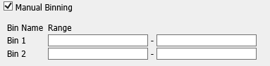
Manual Binning
For Dependent and Stratification variables: Select the Manual Binning checkbox if you want to bin manually.

Note

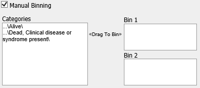
This is the only binning method available if you want to bin a categorical variable.

Complete the binning form that populates as a result of checking the Manual Binning box.
- For continuous data:
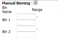
- For categorical data:

Data Binning Using Survival Analysis¶

Data binning is used in survival analyses if the variable you want to use is continuous (for example, age) but needs to be viewed as categorical data. Alternatively, binning can be used to regroup categorical data to consider it as a single variable. For example, if histological grade with values such as Well Defined, Moderately Well Defined, and Poorly Defined are selected, you can group Moderately Well Defined with Poorly Defined and treat them as one group for the purposes of this analysis.

To use the data binning feature with a survival analysis:

Begin to set up a Survival Analysis by following the instructions in section Survival Analysis.
Enable binning by selecting Enable binning.
Define the following and then click Run.
Variable Type

Select whether the variable you have defined above is continuous or categorical.

A continuous variable can be treated as a categorical variable when you use the binning feature.

Number of Bins

Type the number of bins you would like data to be organized in.

This step may require trial and error based on how you want to display data.

Bin Assignments
Select how you would like data to be binned.

Note

This feature can only be used when the variable type selected above is continuous.
- Evenly Distribute Population: Assigns bins based on the underlying data.
  
  For example, if the majority of the subjects in the study were elderly, bins based on age could look like: [(1-40), (40-80), (81-85), (86-90), (90-92)].
- Evenly Spaced Bins: Creates bins based on the overall range of the variable.
  
  For example, if the majority of the subjects in the study were elderly, bins based on age could look like: [(1-20), (21-40), (41-60), (61-80), (81-100)].
Manual Binning
Select the checkbox if you want to bin manually.

Note

This is the only binning method available if you are trying to bin a categorical variable type.

Complete the binning form that populates as a result of checking the Manual Binning box.
- For continuous data:
- For categorical data:

Data Binning Using Table with Fisher Test¶

Data binning is used in Fisher Test analyses if the variable you want to use is continuous (for example, age) but needs to be viewed as categorical data. Alternatively, binning can be used to regroup categorical data to consider it as a single variable. For example, if histological grade with values such as Well Defined, Moderately Well Defined, and Poorly Defined are selected, you can group Moderately Well Defined with Poorly Defined and treat them as one group for the purposes of the analysis.

To use the data binning feature with a Fisher Test analysis:

Begin to set up a Table with Fisher Test analysis by following the instructions in section Table with Fisher Test.
Enable binning by selecting Enable binning.
Define the following and then click Run.
Variable

Select the variable(s) you want to bin by checking the Bin the [*variableType*] Variable box next to the appropriate variables. You can bin from none to both variables.

Example for binning an independent variable:

Variable Type

Select whether the variable you have defined above is continuous or categorical.

A continuous variable can be treated as a categorical variable when you use the binning feature.

Number of Bins

Type the number of bins you would like data to be organized in.

This step may require trial and error based on how you want to display data.

Bin Assignments
Select how you would like data to be binned.

Note

This feature can only be used when the variable type selected above is continuous.
- Evenly Distribute Population: Assigns bins based on the underlying data.
  
  For example, if the majority of the subjects in the study were elderly, bins based on age could look like: [(1-40), (40-80), (81-85), (86-90), (90-92)].
- Evenly Spaced Bins: Creates bins based on the overall range of the variable.
  
  For example, if the majority of the subjects in the study were elderly, bins based on age could look like: [(1-20), (21-40), (41-60), (61-80), (81-100)].
Manual Binning
Select the checkbox if you want to bin manually.

Note

This is the only binning method available if you are trying to bin a categorical variable type.

Complete the binning form that populates as a result of checking the Manual Binning box.
- For continuous data:
- For categorical data:

Running Across-Trial Analyses¶

You run analyses based on cohorts defined from the Across Trials folder just as you do analyses based on cohorts defined from single-study folders.

Viewing Recent Analysis Jobs¶

The Analysis Jobs tab allows you to review analyses you have run previously, and also to see the status of analyses you have chosen to run in the background.

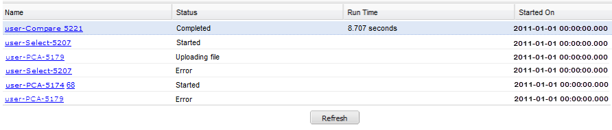
Each advanced workflow that you have run in the past seven days is logged in the Jobs tab in a spreadsheet format.

The columns of information in the Analysis Jobs tab are described below:

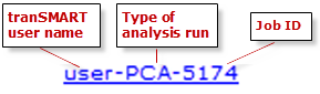
Name

The name of the analysis run. The format of the name is as follows:

Status

The status of the analysis. Statuses are explained below:

Completed — The job has finished and a visualization is available.

Started — The job has been started and is still processing.

Uploading File — You have selected to load additional data into your visualization, and the data is still in the process of uploading to tranSMART.

Error — The job did not complete due to an error.

Cancelled — The job was cancelled and will not complete.

Run Time

The time the analysis took to process.

Started On

The date and time that the analysis was first started.

Note

Click the Refresh button to view any changes that have been made since the Analysis Jobs tab initially populated:

Viewing a Logged Job¶

Each advanced analysis that you have run in the previous seven days will be logged in the Analysis Jobs tab. You may view the visualization again by selecting it from the list.

To run a logged advanced workflow:

In Analyze, click the Analysis Jobs tab:
Click the hyperlink of the analysis you are interested in viewing:

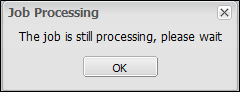
If you click on a job that has not been completed, the following dialog box appears:

Z-score calculation¶

The z-scores used by default in the advanced analysis like the Heatmaps are calculated during the data loading and are dependent on the ETL tool used to load the data. It is recommended to check the documentation of your ETL tool for more information on this. Documentation for transmart-batch.

Some of the advanced analysis that use the z-score have a check box to indicate Calculate z-score on the fly. This uses the log transformed representation of the data to recalculate the z-score based on the subset of data that was selected. The z-score is calculated using the following formula:

\[z-score = \frac{X - \mu}{\sigma} = \frac{probe\_value - probe\_median}{probe\_stdev}\]

If the standard deviation of the probe is 0 the z-score will be equal to 0. The final z-score will be cut-off with a minimum value of -2.5 and a maximum value of 2.5.

The median that is used in the calculation is retrieved from the subset of the data you selected and the z-score calculation takes into consideration the subset a patient is in. In practice this means when using two subsets in your analysis the median value for the probe will be different between these two groups.

Value	0	1	2	3
Counts	120	14	4	2

	Value	0	1	2	3
Bin
1		70	0	0	0
2		35	0	0	0
3		0	0	0	0
4		15	14	4	2

Table Of Contents

Advanced Workflows¶

Running the Analyses¶

aCGH Survival Analysis¶

Box Plot with ANOVA¶

Correlation Analysis¶

Forest Plot¶

Frequency Plot for aCGH¶

GenePrint¶

Group Test for aCGH¶

Group Test for RNASeq¶

Heatmaps¶

Max rows to display¶

Selecting biomarker subsets¶

Standard Heatmap¶

Hierarchical Clustering¶

K-Means Clustering¶

Marker Selection¶

IC50 Dose Response Curve¶

Line Graph¶

Logistic Regression¶

PCA¶

Scatter Plot with Linear Regression¶

Log10 Transformation¶

Survival Analysis¶

Table with Fisher Test¶

Table with Fisher Test with Linked Events¶

Waterfall Plot¶

High Dimensional Data¶

Data Binning¶

Data binning caveats¶

Data Binning Using Box Plot with ANOVA¶

Data Binning Using Forest Plot¶

Data Binning Using Survival Analysis¶

Data Binning Using Table with Fisher Test¶

Running Across-Trial Analyses¶

Viewing Recent Analysis Jobs¶

Viewing a Logged Job¶

Z-score calculation¶

Log₁₀ Transformation¶